NBA Player Evaluation Using Ridge Regression and the Lasso

DATA622-Lab4

In this lab you are going to be using resampling techniques (cross-validation and the bootstrap) along with regularization (ridge regression and the lasso) to rank basketball players based on their performance during the 2022 NBA season. To get the most out of this lab, you do not need to be an expert on the NBA, but you do need to pay attention to the following background information.

Basketball is a sport played between two teams. Each team has 12 total players, but only 5 are on the court for each team at a given time. The goal of the game is to score more points than the other team during the 48 minutes of game time. Points are scored by “shooting” a ball into a 10 foot tall metal hoop called the “basket”. If you want to watch the gameplay, [skim this video]. Or, you can watch [this 8 minute video that explains the rules].

Traditionally, basketball players have been evaluated based on their individual statistics, such as the number of points that they score in a game, the number of “rebounds” they get (a rebound is when a player catches the ball after a missed shot), the number of “steals” (when a player takes the ball from the other team), and more. However, basketball is a complicated team sport, and the actions of all five players on a team contribute to these individual statistics.

The goal of capturing these more abstract contributions to success has led to the concept of “plus-minus”, which looks at how the presence or absence of a player on the court correlates with the scoring margin of the team. The idea is to model what happens in a basketball game by assigning each player on both teams a “coefficient”, which will be called “RAPM” during this homework assignment. “RAPM” stands for Regularized Adjusted Plus Minus, and it measures the contribution of each player to the expected point differential between the two teams. A player with a RAPM of 3 is expected to add 3 points to their team’s net performance for every 100 possessions of a basketball game (a possession is defined as a period of the game where a single team has control of the ball, games consist of a series of alternating possessions and there are usually about 200 possessions in a game, 100 per team).

Suppose that two teams are playing against each other, and that the “lineups” of the two teams stay the same for a certain number of possessions, call it num_pos. This period of time with constant lineups is called a stint, and we can model the probability distribution for the point “margin”, defined as:

\[ (\mathrm{points\_home} - \mathrm{points\_road})\cdot \frac{100}{\mathrm{n\_pos}} \]

in the ‘stint’ using the following formula:

\[ \mathrm{margin}_i \sim \mathrm{Normal}\left(\sum_{j} c_{ij}\left(\mathrm{RAPM}\right)_j, \sigma^2 \right) \]

Here, the sum is over all the different players in the dataset, and the coefficient $c_{ij}$ is +1 if that player $j$ was on the court during stint $i$ and playing for the “home” team, and -1 if they were on the court for the “road” team. The coefficient is $0$ otherwise. The “home” team and “road” team distinction allows us to use the same data for players who were playing against each other. The “margin” variable is the point differential during the stint normalized to points per 100 possessions.

The dataset to fit this model is contained in [nba_stint_data.csv]

Let’s take a look at it:

stints.head(10)

	game_id	stint_id	n_pos	home_points	away_points	minutes	margin	201939	202691	203110	...
0	22200002	1	14	5	2	2.70	21.428571	1	1	1	...
1	22200002	2	9	6	2	1.67	44.444444	1	1	1	...
2	22200002	3	5	0	3	0.48	-60.000000	1	0	1	...
3	22200002	4	5	5	1	0.78	80.000000	1	0	1	...
4	22200002	5	9	3	6	1.52	-33.333333	1	0	0	...
5	22200002	6	8	0	6	1.45	-75.000000	1	0	0	...
6	22200002	7	5	0	0	0.80	0.000000	0	0	0	...
7	22200002	8	5	1	0	0.90	20.000000	0	0	0	...
8	22200002	9	3	2	0	0.97	66.666667	0	0	0	...
9	22200002	10	7	2	2	1.66	0.000000	1	0	0	...

10 rows × 546 columns

Here you can see that each row corresponds to a stint where the players on the court didn’t change. The n_pos variable is the number of possessions that took place during that stint. The home_points and away_points are the number of points scored by the home and away teams respectively. The minutes describes how long in minutes the stint lasted, and the margin is the target variable (defined earlier). The features in column 7 onwards are labeled by player ids, and the value in each cell corresponds to the $c_i$ values for that stint (whether the player was on the court for the home team, road team, or neither). You can recover the identity of the players from the [player_id] file.

In the following you will be exploring different ways of calculating the the RAPM model coefficients and interpreting them in terms of player skill.

Problem 1: Ridge Regression for Inference

Ordinary Linear Regression:

Use ordinary linear regression to fit the model described in the overview. Use cross-validation to estimate the out of sample root mean squared error and compare it to the in sample error, you may use RidgeCV with $alpha=1e-8$ to keep consistency with the rest of the assignment, or use LinearRegression. Make sure fit_intercept=True, the intercept corresponds to the home court advantage, and do not use sample_weight.

Does the difference between in-sample and cross-validated mean squared error suggest a major problem with overfitting?

Prep:

The target (y variable) is $margin and the predictors are the player, everything past column 7.

x=stints.iloc[:,7:]
y= stints["margin"]

Fit the Linear Model:

m1= linear_model.LinearRegression(fit_intercept=True)
results=m1.fit(x, y)

Comparing MSE

#-- In sample--
y_p= m1.predict(x)
mse_insamp= mean_squared_error(y, y_p)

#--cross-validated--
cv= cross_val_score(m1, x, y, scoring="neg_mean_squared_error")
cv= -cv.mean()

print(f"In-Sample MSE:{mse_insamp}")
print(f"Cross-Validated MSE:{cv}")

In-Sample MSE:4848.181932061575
Cross-Validated MSE:5132.395505838158

The in-sample mean squared error was lower than the cross validated. The error is because the predictions come directly from the training datapoints. The values are pretty close to each other, I can’t say there’s an overfitting problem here but by the nature of the in-sample measurement I would always expect it to be lower than the cross validated.

Examining `RAPM` Coefficients:

Create a dataframe with the player-ids, the RAPM coefficients, and join it with the player names (from the data file shared earlier).

Use the stint matrix to calculate the number of minutes that each player played (minutes variable) and add that to the data frame too.

Sort the players in descending order by ‘RAPM’ and print the top 20 players by ‘RAPM’. What do you notice about their minutes played? Look up the names of a few of the top players on the internet- are they regarded as top NBA players?

Make a scatter plot of RAPM versus minutes-played.

#--Player id df--
players= pd.read_csv("https://raw.githubusercontent.com/georgehagstrom/DATA622Spring2026/refs/heads/main/website/assignments/labs/labData/player_id.csv")

#--Model RAPM Coefficients--
rapm=dict(zip(players["player_id"].astype(int), m1.coef_))
players["rapm"]= players["player_id"].map(rapm)

#--Join Stints--
#stint matrix
stints2= stints.iloc[:,7:]
minutes= stints["minutes"].values

#-- using absolute value because of the "road" -1s--
stints2= abs(stints2).T

#--Calculate minutes--
players2= (stints2 * stints["minutes"].values).sum(axis=1)
players2=players2.to_frame(name= "t_minutes")
players2.index.name= "player_id"
players2= players2.reset_index().astype(int)

#-- Joining on players--
players= players.merge(players2, on="player_id", how= "left")
players= players.sort_values("rapm", ascending= False)

The player matrix stint x player, transposed, becomes player x stint. In this shape, I could multiply the array of minutes to produce the minutes played per stint.

Player Top 20 Lineup

#-- The players have a headshot and the ID's are real!-- 
top20=pd.DataFrame(players.head(20))

top20= top20.copy()

#-- adding the ids to the base url--
top20["image_url"]= top20["player_id"].astype(str).apply(lambda x: f"https://cdn.nba.com/headshots/nba/latest/1040x760/{x}.png")

header= "<h1 style='text-align:center;'>Top 20 by RAPM</h1>"
p_cards = "".join(
    f"<div style='text-align:center;'>"
    f"<img src='{row.image_url}' style='width:90px;'>"
    f"<div style= 'font-size:13px;'>{row.player_name}</div>"
    f"<div style= 'font-size:12px;'>RAPM: {row.rapm:.3f}</div>"
    f"<div style= 'font-size:12px;'>Play Time: {row.t_minutes}</div>"
    f"</div>"
    for player, row in top20.iterrows())
    
HTML(f"<div style='display:grid;grid-template-columns:repeat(5,1fr); gap:8px;'>{p_cards}</div>")

Gabe York

RAPM: 77.399

Play Time: 53

Theo Pinson

RAPM: 62.877

Play Time: 316

Zach LaVine

RAPM: 50.272

Play Time: 2783

Isaiah Stewart

RAPM: 50.138

Play Time: 1332

Delon Wright

RAPM: 47.435

Play Time: 1234

Trae Young

RAPM: 47.427

Play Time: 2706

Chris Silva

RAPM: 41.990

Play Time: 7

Nikola Jovic

RAPM: 37.628

Play Time: 167

Jericho Sims

RAPM: 37.509

Play Time: 802

Danuel House Jr.

RAPM: 36.865

Play Time: 830

James Wiseman

RAPM: 36.223

Play Time: 785

Mark Williams

RAPM: 36.063

Play Time: 816

Jeremy Sochan

RAPM: 34.273

Play Time: 1263

Julius Randle

RAPM: 33.438

Play Time: 2956

Joe Wieskamp

RAPM: 33.412

Play Time: 41

Jaden Springer

RAPM: 33.313

Play Time: 89

Andre Iguodala

RAPM: 33.030

Play Time: 116

Bryce McGowens

RAPM: 33.015

Play Time: 820

Aaron Wiggins

RAPM: 32.954

Play Time: 1221

Omer Yurtseven

RAPM: 32.606

Play Time: 76

I’m not familiar with the NBA, but I can accurately say Lebron James is not in this lineup. On a side note, the resulting top 20 do share low play time so the high RAPM scores might be assigned to players who don’t play for very long.

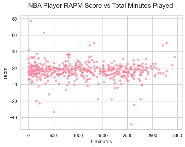
#-- fixing sns--
sns.set_theme(style="whitegrid", palette= "husl")
plt.rcParams["axes.titlesize"] = 16
plt.rcParams["axes.titlepad"] = 20

#-- Visualize RAPM--
sns.scatterplot(data= players, x="t_minutes", y="rapm", alpha= 0.6)
plt.title("NBA Player RAPM Score vs Total Minutes Played ")
plt.show()

The scatterplot shows the linear relationship between rapm and t_minutes is basically zero.

Ridge Regression RAPM:

The results of (b) suggest that the model is attaching extreme values of RAPM to low minute players, something which can be potentially fixed with regularization. Define a vector of regularization parameters alpha on a logarithmic scale between $10^{-2}$ and $10^{5}$ (look up np.logspace).

Make this vector contain at least 10 but not more than 200 values of alpha (pick based on how fast your computer is). Use RidgeCV to fit a ridge regression model, selecting the model with the best value of the hyperparameters.

What value of alpha is optimal? Next, repeat the same calculation as you did in part (b) (you could create a function or just copy the dataframe and replace the old RAPM with new RAPM). Look up some of the top players that your model identified, are they well regarded by the NBA?

Make a scatterplot of RAPM versus minutes played.

Fitting Rdige Model & Alpha Range

alpha= np.logspace(-2, 5, 50)
m2= RidgeCV(alphas=alpha, fit_intercept= True, cv=5)
m2.fit(x,y)

RidgeCV(alphas=array([1.00000000e-02, 1.38949549e-02, 1.93069773e-02, 2.68269580e-02,
       3.72759372e-02, 5.17947468e-02, 7.19685673e-02, 1.00000000e-01,
       1.38949549e-01, 1.93069773e-01, 2.68269580e-01, 3.72759372e-01,
       5.17947468e-01, 7.19685673e-01, 1.00000000e+00, 1.38949549e+00,
       1.93069773e+00, 2.68269580e+00, 3.72759372e+00, 5.17947468e+00,
       7.19685673e+00, 1.00000000e+0...
       2.68269580e+01, 3.72759372e+01, 5.17947468e+01, 7.19685673e+01,
       1.00000000e+02, 1.38949549e+02, 1.93069773e+02, 2.68269580e+02,
       3.72759372e+02, 5.17947468e+02, 7.19685673e+02, 1.00000000e+03,
       1.38949549e+03, 1.93069773e+03, 2.68269580e+03, 3.72759372e+03,
       5.17947468e+03, 7.19685673e+03, 1.00000000e+04, 1.38949549e+04,
       1.93069773e+04, 2.68269580e+04, 3.72759372e+04, 5.17947468e+04,
       7.19685673e+04, 1.00000000e+05]),
        cv=5)

In a Jupyter environment, please rerun this cell to show the HTML representation or trust the notebook.
On GitHub, the HTML representation is unable to render, please try loading this page with nbviewer.org.

Optimal Value of Alpha

print(f"Optimal Value of alpha: {m2.alpha_.round(2)}")

Optimal Value of alpha: 719.69

Model 2 Player Top 20 Lineup

#--pulling the ridge values--
rapm2=dict(zip(players["player_id"].astype(int), m2.coef_))
players["rapm2"]= players["player_id"].map(rapm2)
players= players.sort_values("rapm2", ascending= False)
top20=pd.DataFrame(players.head(20))
top20= top20.copy()

#-- adding the ids to the base url--
top20["image_url"]= top20["player_id"].astype(str).apply(lambda x: f"https://cdn.nba.com/headshots/nba/latest/1040x760/{x}.png")

header= "<h1 style='text-align:center;'>Model 2: Top 20 by RAPM (Ridge)</h1>"
p_cards = "".join(
    f"<div style='text-align:center;'>"
    f"<img src='{row.image_url}' style='width:90px;'>"
    f"<div style= 'font-size:13px;font-weight: bold'>{row.player_name}</div>"
    f"<div style= 'font-size:12px;'>RAPM: {row.rapm2:.3f}</div>"
    f"<div style= 'font-size:12px;'>Play Time: {row.t_minutes}</div>"
    f"</div>"
    for player, row in top20.iterrows())
    
HTML(f"<div style='display:grid;grid-template-columns:repeat(5,1fr); gap:8px;'>{p_cards}</div>")

Chuma Okeke

RAPM: 5.653

Play Time: 513

Clint Capela

RAPM: 4.916

Play Time: 1696

Cam Reddish

RAPM: 4.692

Play Time: 957

Keita Bates-Diop

RAPM: 4.258

Play Time: 1318

Tyrese Maxey

RAPM: 3.862

Play Time: 2000

Collin Sexton

RAPM: 3.852

Play Time: 1192

Zach LaVine

RAPM: 3.761

Play Time: 2783

Brook Lopez

RAPM: 3.516

Play Time: 2156

George Hill

RAPM: 3.506

Play Time: 892

Jalen Green

RAPM: 3.385

Play Time: 2575

Kevin Love

RAPM: 3.364

Play Time: 1131

Rui Hachimura

RAPM: 3.353

Play Time: 1504

Andre Iguodala

RAPM: 3.302

Play Time: 116

Jock Landale

RAPM: 3.279

Play Time: 921

Jeff Dowtin Jr.

RAPM: 3.266

Play Time: 238

Nathan Knight

RAPM: 3.220

Play Time: 312

Justin Champagnie

RAPM: 3.118

Play Time: 22

Malachi Flynn

RAPM: 3.027

Play Time: 658

Malik Monk

RAPM: 2.952

Play Time: 1678

OG Anunoby

RAPM: 2.951

Play Time: 2287

Problem 2: Possession Weights

Heteroscedasticity in Stints:

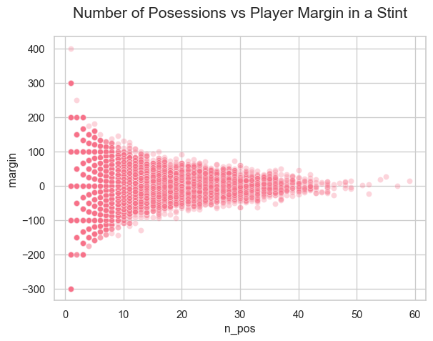
Make a plot of the margin variable as a function of the number of possessions in a stint. What do you notice about the variance of margin? Why do you think it is happening?

The plot below is a funnel shape, it goes from wide variance to low variance. It seems symmetrical if sliced at zero. It is an example pf heteroscedasticity as the variance is not constant but seems to have a pattern.

sns.scatterplot(data=stints, x="n_pos", y="margin", alpha= 0.3)
plt.title("Number of Posessions vs Player Margin in a Stint")
plt.show()

Implementing Weights Regression:

The solution to the issue that you observed in 2(a) is something called weighted least squares This involves adjusting the error term for each stint, based on a weight that accounts for whatever factor controls the variance.

The new weighted model looks like this:

\[ \mathrm{margin}_i \sim \mathrm{Normal}\left(\sum_{j} c_{ij}\left(\mathrm{RAPM}\right)_j, \frac{\sigma^2}{w_i} \right) \]

where $w_i$ is a coefficient that determines how the variance of margin should scale for each stint. The idea is that $w_i$ should be smaller for stints where the variance is high, and larger for stints where the variance is low. This forces the model to fit the low-variance stints more closely than the high-variance stints. The correct weights for this problem are the $w_i = \mathrm{num\_pos}_i$, which implies that the variance of the margin is inversely proportional to the number of stints.

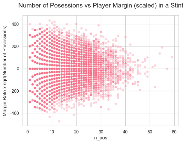
Verify this by making a scatter plot of the margin rate times the square root of the number of possessions versus the number of possessions.

Then recalculate the player RAPM coefficients from 1(c) by setting the weights keyword in the model fit to be n_pos. How have the rankings of top players changed?

Scatterplot for Scaled Margin

sns.scatterplot(data=stints, x="n_pos", y=stints["margin"] * np.sqrt(stints["n_pos"]), alpha= 0.3)
plt.title("Number of Posessions vs Player Margin (scaled) in a Stint")
plt.ylabel("Margin Rate x sqrt(Number of Posessions)")
plt.show()

RAPM Recalculation

#-- weights keyword--
m3= RidgeCV(alphas=alpha, fit_intercept= True)
m3.fit(x,y, sample_weight= stints["n_pos"])

#--pulling the ridge values--
rapm3=dict(zip(x.columns.astype(int), m3.coef_))
players["rapm3"]= players["player_id"].map(rapm3)
players= players.sort_values("rapm3", ascending= False)
top20=pd.DataFrame(players.head(20))
top20= top20.copy()

Model 3 Player Top 20 Lineup

#-- adding the ids to the base url p3--
top20["image_url"]= top20["player_id"].astype(str).apply(lambda x: f"https://cdn.nba.com/headshots/nba/latest/1040x760/{x}.png")

header= "<h1 style='text-align:center;'>Model 3: Top 20 by RAPM</h1>"

p_cards = "".join(
    f"<div style='text-align:center;'>"
    f"<img src='{row.image_url}' style='width:90px;'>"
    f"<div style= 'font-size:13px;font-weight: bold'>{row.player_name}</div>"
    f"<div style= 'font-size:12px;'>RAPM: {row.rapm3:.3f}</div>"
    f"<div style= 'font-size:12px;'>Play Time: {row.t_minutes}</div>"
    f"</div>"
    for player, row in top20.iterrows())
    
HTML(f"<div style='display:grid;grid-template-columns:repeat(5,1fr); gap:8px;'>{p_cards}</div>")

Nikola Jokic

RAPM: 2.782

Play Time: 2255

Draymond Green

RAPM: 2.645

Play Time: 2019

Joel Embiid

RAPM: 2.558

Play Time: 2249

Jrue Holiday

RAPM: 2.495

Play Time: 2097

Kawhi Leonard

RAPM: 2.295

Play Time: 1817

Giannis Antetokounmpo

RAPM: 2.274

Play Time: 1840

Aaron Gordon

RAPM: 2.097

Play Time: 1966

Anthony Davis

RAPM: 2.093

Play Time: 1880

Josh Hart

RAPM: 2.073

Play Time: 2474

Brook Lopez

RAPM: 1.885

Play Time: 2156

Christian Koloko

RAPM: 1.883

Play Time: 757

Derrick White

RAPM: 1.833

Play Time: 2078

Zion Williamson

RAPM: 1.821

Play Time: 859

Michael Porter Jr.

RAPM: 1.787

Play Time: 1686

Jayson Tatum

RAPM: 1.725

Play Time: 2771

Desmond Bane

RAPM: 1.702

Play Time: 1706

Nicolas Batum

RAPM: 1.577

Play Time: 1814

Austin Reaves

RAPM: 1.534

Play Time: 1901

Jarrett Allen

RAPM: 1.488

Play Time: 2076

Devin Booker

RAPM: 1.434

Play Time: 1904

Problem 3: Interpreting Bootstrap Uncertainty

Calculate Confidence Intervals Using the Bootstrap:

Suppose you are a general manager for a basketball team. You want to identify candidate players to add to your team, but you are unsure how certain to be about the ‘RAPM’ coefficients for the model. The bootstrap is a standard approach for calculating confidence intervals for model coefficients.

Use either the resample function from sklearn or np.random.choice along with a loop to calculate bootstrap samples of the model coefficients for each player. You may use the optimal alpha found during the hyperparameter search in 2(b) for all bootstrap fits.

Do not forget to resample the weights when bootstrapping!

For the top 20 players, display the RAPM estimates along with the confidence interval (calculate 92% intervals or some other high value that isn’t 95%). How much do the intervals of the top 20 overlap?

Boot Loop

boot_ridge= Ridge(alpha=m3.alpha_, fit_intercept=True)
boot_ridge.fit(x, y, sample_weight=stints["n_pos"])

#--calculating bootstrap samples--
boot=[]

for a in range(400):
  sampled= np.random.choice(len(y), size=len(y), replace=True)
  
  x_a= x.iloc[sampled]
  y_a= y.iloc[sampled]
  z_b= stints["n_pos"].values[sampled]
  
  m4= Ridge(alpha= m2.alpha_, fit_intercept=True)
  m4.fit(x_a, y_a, sample_weight= z_b)
  boot.append(m4.coef_)

boot= np.array(boot)

Player CI: Upper and Lower at 92%

#--matching the Player IDs--
rapm4=dict(zip(x.columns.astype(int), m4.coef_))
cil_map= dict(zip(x.columns.astype(int), np.percentile(boot, 4, axis=0)))
ciu_map= dict(zip(x.columns.astype(int), np.percentile(boot, 96, axis=0)))

#-- Adding the Cis
players= players.copy()

players["rapm4"]= players["player_id"].map(rapm4)
players["ci_lower"]= players["player_id"].map(cil_map)
players["ci_upper"]= players["player_id"].map(ciu_map)

players= players.sort_values("rapm4", ascending=False)
top20= players.head(20).copy()
top20["ci_range"]= top20["ci_upper"]-top20["ci_lower"]

Model 4 Player Top 20 Lineup

#-- adding the ids to the base url p3--
top20["image_url"]= top20["player_id"].astype(str).apply(lambda x: f"https://cdn.nba.com/headshots/nba/latest/1040x760/{x}.png")

header= "<h1 style='text-align:center;'>Model 4: Top 20 by RAPM (after Bootstrapping)</h1>"

p_cards = "".join(
    f"<div style='text-align:center;'>"
    f"<img src='{row.image_url}' style='width:90px;'>"
    f"<div style= 'font-size:14px; font-weight: bold'>{row.player_name}</div>"
    f"<div style= 'font-size:12px;'>RAPM: {row.rapm4:.3f}</div>"
    f"<div style= 'font-size:12px;'>CI Lower: {row.ci_lower:.3f}</div>"
    f"<div style= 'font-size:12px;'>CI Upper: {row.ci_upper:.3f}</div>"
    f"<div style= 'font-size:14px; font-weight: bold'>CI Range:{row.ci_range:.3f}</div>"
    f"</div>"
    for player, row in top20.iterrows())
    
HTML(f"<div style='display:grid;grid-template-columns:repeat(5,1fr); gap:8px;'>{p_cards}</div>")

Nikola Jokic

RAPM: 7.424

CI Lower: 3.999

CI Upper: 10.605

CI Range:6.605

Jrue Holiday

RAPM: 7.296

CI Lower: 1.977

CI Upper: 7.692

CI Range:5.715

Alex Len

RAPM: 7.291

CI Lower: -0.894

CI Upper: 6.288

CI Range:7.182

Charles Bassey

RAPM: 6.834

CI Lower: 0.617

CI Upper: 7.002

CI Range:6.385

Kawhi Leonard

RAPM: 6.478

CI Lower: 2.378

CI Upper: 8.260

CI Range:5.883

Moses Moody

RAPM: 6.429

CI Lower: -0.806

CI Upper: 5.624

CI Range:6.430

Draymond Green

RAPM: 5.771

CI Lower: 3.029

CI Upper: 9.432

CI Range:6.403

Joel Embiid

RAPM: 5.576

CI Lower: 3.522

CI Upper: 8.899

CI Range:5.378

Jarrett Allen

RAPM: 5.524

CI Lower: -0.183

CI Upper: 5.559

CI Range:5.741

George Hill

RAPM: 5.389

CI Lower: -2.154

CI Upper: 4.543

CI Range:6.697

Luka Samanic

RAPM: 5.296

CI Lower: 0.232

CI Upper: 7.728

CI Range:7.496

Zach Collins

RAPM: 5.230

CI Lower: 0.996

CI Upper: 6.911

CI Range:5.915

Anthony Davis

RAPM: 5.224

CI Lower: 3.274

CI Upper: 9.180

CI Range:5.905

Steven Adams

RAPM: 5.066

CI Lower: -0.117

CI Upper: 5.843

CI Range:5.960

Marko Simonovic

RAPM: 5.031

CI Lower: -1.783

CI Upper: 3.852

CI Range:5.635

Oshae Brissett

RAPM: 4.982

CI Lower: -1.123

CI Upper: 5.442

CI Range:6.565

Boban Marjanovic

RAPM: 4.967

CI Lower: 2.207

CI Upper: 9.489

CI Range:7.282

Shaquille Harrison

RAPM: 4.894

CI Lower: -1.617

CI Upper: 4.978

CI Range:6.595

Carlik Jones

RAPM: 4.836

CI Lower: -2.177

CI Upper: 4.455

CI Range:6.633

Hamidou Diallo

RAPM: 4.707

CI Lower: -1.697

CI Upper: 3.942

CI Range:5.639

There is an overlap here in the Top 20

Impact of Minutes Played on Confidence Intervals:

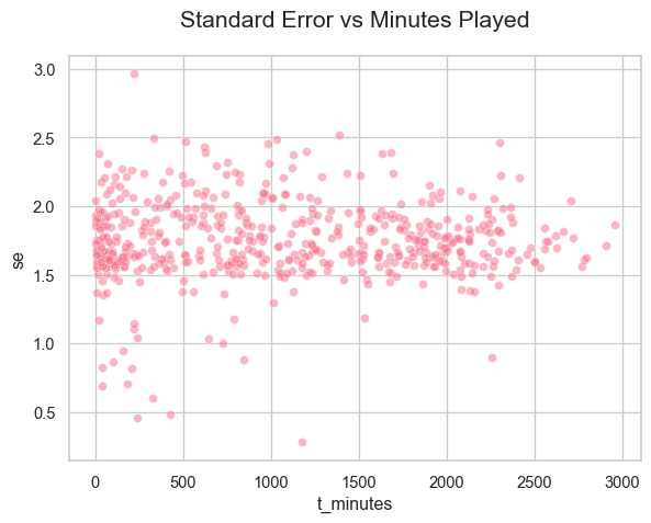
One potential use of a model like this is to find players who do not play much but who might do well with more opportunity. Calculate the standard errors of each coefficient from the bootstrap samples and make a scatterplot of standard error versus minutes played.

Comment on the relationship between minutes played and standard error- does it make sense to you intuitively and/or statistically?

players["se"]=np.std(boot, axis=0)

sns.scatterplot(data=players, x="t_minutes", y="se", alpha=0.5)
plt.title("Standard Error vs Minutes Played")
plt.show()

The plot is not as dramatic as the funnel earlier but there is still many differences in variation on t_minues so there is heteroscaticity here. The relationship between se and t_minutes is not strong, but with the alpha at 0.4 I can notice that the points that overlap have a little curve. Maybe theres a nonlinear relationship? I’m not sure.

Comparison to Bayesian Credible Intervals:

Bayesian statistics (which you should have learned about briefly in DATA 606) is a field of statistics based on an interpretation of probability as referring to uncertainty about the real world rather than as the frequency of outcomes in repeated experiments. In the Bayesian framework, it is normal to talk about the probability distribution of model parameters, which leads to the concept of a credible interval, defined as an interval with a certain probability of containing the model parameter (a 92% credible interval would have a 92% chance of containing the model parameter). Credible intervals often correspond closely to confidence intervals captured using standard statistics, but this problem is one case where they diverge sharply.

Ridge regression has an interpretation in Bayesian statistics, where the regularization parameter corresponds to the strength of a prior belief that the model coefficients have a normal distribution centered around zero and with variance inversely proportional to the regularization penalty $\alpha$.

For ridge regression interpreted as Bayesian statistics, there is an exact formula for the standard errors and confidence intervals which we can use to contrast with the bootstrap estimate. I have provided code below to calculate the standard errors and the Bayesian credible intervals (if you are curious about the full details [read this article].

Use the code below and calculate the Bayesian standard errors for each ‘RAPM’ coefficient. Make a plot of the Bayesian standard errors versus minutes played and compare to the standard errors calculated from the bootstrap. In which part of the range is the agreement highest? In which part is the disagreement highest? Focusing on the areas where the disagreement is highest, put yourself in the shoes of someone using the model and discuss which estimate of uncertainty is more realistic and why.

(You will need to adapt the code below to your variable names and data structures.)

Code to calculate standard errors and Bayesian credible intervals

# Here MarginVector is your Target
# StintMatrix are your observations
# WeightVector are your weights
# model_ridge is your selected model

# alpha_opt is the optimal regularization parameter from cross validation
x = stints.iloc[:,7:] 
y = stints["margin"]
model_ridge = Ridge(alpha=m2.alpha_, fit_intercept=True)
model_ridge.fit(x, y, sample_weight=stints["n_pos"])

weights = stints["n_pos"].to_numpy() # Need to do this is WeightVector is a pandas series or df etc
stint_mat = stints.iloc[:,7:] # Ditto
margin_vec = stints["margin"] # Ditto
alpha_opt= m2.alpha_


var = np.average((margin_vec - model_ridge.predict(stint_mat))**2, weights=weights) # We need to incorporate weights into variance calculation
num_players = stint_mat.shape[1]

AMat = (stint_mat * weights.reshape(-1, 1)).T @ stint_mat + alpha_opt * np.eye(num_players)

# This is the covariance matrix. You could find very high covariance between players on the same teams

posterior_covariance = var * np.linalg.inv(AMat) 

se_vec = np.sqrt(np.diag(posterior_covariance)) #These are the standard errors

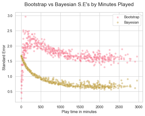
se_boot= np.std(boot, axis=0, ddof=1)
se_boot_map= dict(zip(x.columns.astype(int), se_boot))
players["se_boot"]= players["player_id"].astype(int).map(se_boot_map)

se_bayes_map = dict(zip(x.columns.astype(int), se_vec))
players["se_bayes"] = players["player_id"].astype(int).map(se_bayes_map)

#--plotting--
sns.scatterplot(data= players, x= "t_minutes", y= "se_boot", alpha= 0.4, label="Bootstrap")
sns.scatterplot(data= players, x= "t_minutes", y= "se_bayes", alpha= 0.4, label="Bayesian")

plt.xlabel("Play time in minutes")
plt.ylabel("Standard Error")
plt.title("Bootstrap vs Bayesian S.E's by Minutes Played")
plt.legend()
plt.show()

The standard error is higher in Bootstrap than Bayesian.

Conclusion

Extra Credit (5 Points): Ridge versus Lasso and Confidence/Credible Interval Calculations

An alternative to ridge regression that is used for variable selection is called the Lasso. The Lasso differs penalty causes a large number of model coefficients to be zero, making it a good tool for variable selection and for creating interpretable models.

Use LassoCV to calculate the RAPM coefficients. I recommend using regularization weights that range between $10^{-4}$ and $10^2$ (the scale needs to be different compared to ridge regression).

Compare the RAPM values calculated with lasso to those calculated with ridge regression. Are there any notable differences in the top 20 players?

Find the 10 players with the largest difference between lasso RAPM and Ridge RAPM in both directions (ridge greater than lasso and lasso greater than ridge). Within the players where there was large disagreement, consider how the players performed in the next NBA season (you may do this however you like, I recommend reading media reports about those players during the next season) and determine which model was more correct when it comes to players with large disagreements.

There is a subtle conceptual flaw in how the confidence or credible intervals were calculated in this lab. This is apparent if you paid very close attention during the meetup. Can you tell me what it is?

#--reg weights-- 
lasso_alpha= np.logspace(-4, 2, 1000)

#--Lasso RAPM Coefficients--
m5= LassoCV(alphas=lasso_alpha, fit_intercept=True)
m5.fit(x,y, sample_weight=stints["n_pos"])

#--Mapping RAPMs--
#ridge
rapm_Ridge= dict(zip(x.columns.astype(int), m4.coef_))
players= players.copy()
players["rapm_Ridge"]= players["player_id"].map(rapm_Ridge)
#lasso
rapm_Lasso=dict(zip(x.columns.astype(int), m5.coef_))
players["rapm_Lasso"]= players["player_id"].map(rapm_Lasso)

players= players.sort_values("rapm_Lasso", ascending= False)
top20=pd.DataFrame(players.head(20))
top20= top20.copy()

top20["image_url"]= top20["player_id"].astype(str).apply(lambda x: f"https://cdn.nba.com/headshots/nba/latest/1040x760/{x}.png")

header= "<h1 style='text-align:center;'>Model 4: Top 20 by RAPM (after Bootstrapping)</h1>"

p_cards = "".join(
    f"<div style='text-align:center;'>"
    f"<img src='{row.image_url}' style='width:90px;'>"
    f"<div style= 'font-size:14px; font-weight: bold'>{row.player_name}</div>"
    f"<div style= 'font-size:12px;'>Ridge: {row['rapm_Ridge']:.3f}</div>"
    f"<div style= 'font-size:12px;'>Laso: {row['rapm_Lasso']:.3f}</div>"
    f"</div>"
    for player, row in top20.iterrows())
    
HTML(f"<div style='display:grid;grid-template-columns:repeat(5,1fr); gap:8px;'>{p_cards}</div>")

Joel Embiid

Ridge: 5.576

Laso: 5.868

Draymond Green

Ridge: 5.771

Laso: 5.863

Nikola Jokic

Ridge: 7.424

Laso: 5.573

Kawhi Leonard

Ridge: 6.478

Laso: 4.400

Anthony Davis

Ridge: 5.224

Laso: 4.220

Christian Koloko

Ridge: 3.084

Laso: 4.080

Jrue Holiday

Ridge: 7.296

Laso: 3.956

Zion Williamson

Ridge: 3.657

Laso: 3.851

Giannis Antetokounmpo

Ridge: 3.989

Laso: 3.488

Cameron Johnson

Ridge: 1.756

Laso: 3.328

Josh Hart

Ridge: 2.266

Laso: 3.180

Derrick White

Ridge: 1.594

Laso: 3.088

Julius Randle

Ridge: 2.536

Laso: 2.999

Jayson Tatum

Ridge: 4.324

Laso: 2.934

Lauri Markkanen

Ridge: 3.206

Laso: 2.602

Desmond Bane

Ridge: 2.654

Laso: 2.597

Shai Gilgeous-Alexander

Ridge: 2.069

Laso: 2.592

Darius Garland

Ridge: 1.457

Laso: 2.567

Aaron Gordon

Ridge: 2.986

Laso: 2.550

Kevin Durant

Ridge: 4.177

Laso: 2.502

The conceptual flaw in how the confidence intervals were calculated might be that there is a bottleneck in the amount of players that can be on the court. Confidence intervals are percentages indicating where an observation falls. There is a cap the probability of being on the court and i don’t think that is accounted for here.

Bibliography

Module 6- Resampling and Cross Validation

https://georgehagstrom.github.io/DATA622Spring2026/modules/module6.html

	alphas alphas: array-like of shape (n_alphas,), default=(0.1, 1.0, 10.0) Array of alpha values to try. Regularization strength; must be a positive float. Regularization improves the conditioning of the problem and reduces the variance of the estimates. Larger values specify stronger regularization. Alpha corresponds to ``1 / (2C)`` in other linear models such as :class:`~sklearn.linear_model.LogisticRegression` or :class:`~sklearn.svm.LinearSVC`. If using Leave-One-Out cross-validation, alphas must be strictly positive.	array([1.0000...00000000e+05])
	fit_intercept fit_intercept: bool, default=True Whether to calculate the intercept for this model. If set to false, no intercept will be used in calculations (i.e. data is expected to be centered).	True
	scoring scoring: str, callable, default=None The scoring method to use for cross-validation. Options: - str: see :ref:`scoring_string_names` for options. - callable: a scorer callable object (e.g., function) with signature ``scorer(estimator, X, y)``. See :ref:`scoring_callable` for details. - `None`: negative :ref:`mean squared error ` if cv is None (i.e. when using leave-one-out cross-validation), or :ref:`coefficient of determination ` (:math:`R^2`) otherwise.	None
	cv cv: int, cross-validation generator or an iterable, default=None Determines the cross-validation splitting strategy. Possible inputs for cv are: - None, to use the efficient Leave-One-Out cross-validation - integer, to specify the number of folds. - :term:`CV splitter`, - An iterable yielding (train, test) splits as arrays of indices. For integer/None inputs, if ``y`` is binary or multiclass, :class:`~sklearn.model_selection.StratifiedKFold` is used, else, :class:`~sklearn.model_selection.KFold` is used. Refer :ref:`User Guide ` for the various cross-validation strategies that can be used here.	5
	gcv_mode gcv_mode: {'auto', 'svd', 'eigen'}, default='auto' Flag indicating which strategy to use when performing Leave-One-Out Cross-Validation. Options are:: 'auto' : use 'svd' if n_samples > n_features, otherwise use 'eigen' 'svd' : force use of singular value decomposition of X when X is dense, eigenvalue decomposition of X^T.X when X is sparse. 'eigen' : force computation via eigendecomposition of X.X^T The 'auto' mode is the default and is intended to pick the cheaper option of the two depending on the shape of the training data.	None
	store_cv_results store_cv_results: bool, default=False Flag indicating if the cross-validation values corresponding to each alpha should be stored in the ``cv_results_`` attribute (see below). This flag is only compatible with ``cv=None`` (i.e. using Leave-One-Out Cross-Validation). .. versionchanged:: 1.5 Parameter name changed from `store_cv_values` to `store_cv_results`.	False
	alpha_per_target alpha_per_target: bool, default=False Flag indicating whether to optimize the alpha value (picked from the `alphas` parameter list) for each target separately (for multi-output settings: multiple prediction targets). When set to `True`, after fitting, the `alpha_` attribute will contain a value for each target. When set to `False`, a single alpha is used for all targets. .. versionadded:: 0.24	False

Problem 1: Ridge Regression for Inference

Ordinary Linear Regression:

Prep:

Fit the Linear Model:

Comparing MSE

Examining RAPM Coefficients:

Player Top 20 Lineup

Ridge Regression RAPM:

Fitting Rdige Model & Alpha Range

Optimal Value of Alpha

Model 2 Player Top 20 Lineup

Problem 2: Possession Weights

Heteroscedasticity in Stints:

Implementing Weights Regression:

Scatterplot for Scaled Margin

RAPM Recalculation

Model 3 Player Top 20 Lineup

Problem 3: Interpreting Bootstrap Uncertainty

Calculate Confidence Intervals Using the Bootstrap:

Boot Loop

Player CI: Upper and Lower at 92%

Model 4 Player Top 20 Lineup

Impact of Minutes Played on Confidence Intervals:

Comparison to Bayesian Credible Intervals:

Conclusion

Extra Credit (5 Points): Ridge versus Lasso and Confidence/Credible Interval Calculations

Bibliography

Examining `RAPM` Coefficients: